I’ve been away for a little while – been incredibly busy with a major work project, which included a lot of hours and travel. Left me too exhausted and with too little time to spend on researching my family tree. However, in May, I came across a blog post that inspired me to spend some time organizing. Michele Simmons Lewis on her blog Ancestoring describes an Excel trick for working with the data in her Ancestry.com family tree. At the end, it produces a spreadsheet with a list of all your ancestors, along with their birth and death dates/places. Part of the beauty of the list is the list of names will contain a hyperlink to the individual profiles on Ancestry.com. Here’s an example of what my list looks like:

My Family List in Excel
Then I took the spreadsheet a few steps further – in part because I’m a complete Excel geek and because I like to use data to solve problems. My next step, I added some extra columns:
Columns in My Spreadsheet
- Relationship (to me)
- Side of the Family (Maternal, Paternal and N/A). N/A is for my siblings, their spouses, children, etc. who don’t belong to actually one side of the family or the other.
- Copies of Citations/Docs Downloaded. (I’ll get more into this below.)
- File location (for the MRIN/Marriage Record Identification Number, which I use for organizing my computer file folders)
In addition to the columns, I do a couple of other things to the data to make it easier to work with:
- Create a table for the range of data. Excel behaves differently when working with data within a table that makes it easier to work with, especially when the data is very similar and when working with formulas. To do this, highlight all the rows and columns of data in the spreadsheet. On the Home tab, select Format as Table, then select the table format that you want/like. I prefer a table that has alternating colors for the lines because I find that easier to read.
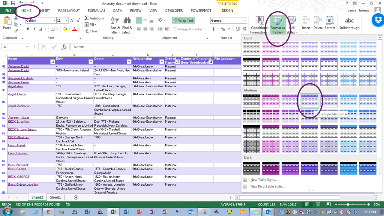
Formatting a Table
- Then I add a Filter to the column headers. Highlight the row of headers, and select Filter on the Data tab. Once the filter is set, you can click on any of the down arrows next to a column header to:
- Sort by that column
- Filter by certain data, such as a surname, and hide all the other rows of data.

Filters in Excel
Once I had the data formatted the way I wanted it, I was ready to get to work. Using the hyperlinked name for each member of my family tree, I noted their relationship to me (concentrating only on direct ancestors and their siblings – I bypassed any cousins x times removed) and what side of the family they fell on. This is easy in the Ancestry.com individual profile, as the relationship is noted in the header information.

Ancestry Profile Header
But the main purpose of this list is to keep track of downloading copies of the records attached to my ancestors’ profiles to my computer to retain my own digital copy of all their records. I’m still working my way through this, but I’ve got a good head start. Once I’ve download the attached records of a particular profile, I mark the row as “Complete” under the column: Copies of Citations/Docs Downloaded. I also save a .pdf of the citation page from Ancestry.com for each record, including any index citations, in the ancestor profile. I then put the path for the file folder on my computer in the last column so that I know where to find these files later.

Download and File Location Columns
The next trick I use in Excel is Conditional Formatting. Whenever I enter the word “Complete” in the Download column, it will highlight the row in green so I can easily see which ancestors I’ve completed downloading the documents for. If the ancestor doesn’t have any source citations in their profile, I mark the column as “None”. Any marked with “None” get highlighted in red.
Conditional Formatting
To use Conditional Formatting to highlight a whole row, based on the contents of a single cell:
- Highlight the row of data.
- Select Conditional Formatting from the Home tab.
- Select New Rule
- In the New Formatting Rule dialog box, select “Use a formula to determine which cells to format”.
- Enter the formula entering an equal sign, click on the cell that will contain the data you want to base the formatting on. In this case, I select the cell F59 for the Download column for row 59. This is where I will note “Complete” or “None”. Enter another equal sign, then the text (in quotes) that you will base the formatting on, in this case, “Complete”.
- Click on the Format… button to select the formatting you want applied to the row, such as fill, font color and border.
- Click OK.
- Repeat the process for “None”.
- Click OK to exit out of the Conditional Formatting dialog box.
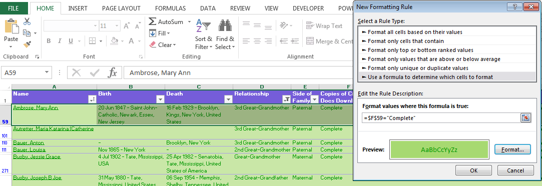
Conditional Formatting Rules
- Select the Format Painter tool and copy the formatting to all rows in the spreadsheet.

Format Painter Tool
Now that the spreadsheet is formatted the way I wanted, I worked my way through my family tree, surname by surname, noting the relationship and side of the family.
Now I can easily produce to do lists for research and downloading records for parts of my family tree by filtering the list based on surname, relationship type, side of the family, etc., depending on what part of my family tree I want to concentrate on.
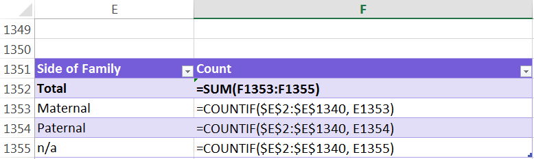
And in the habit of playing with data, I also created some fun tables of summary information at the bottom of my spreadsheet, using some easy Countif formulas:
Counts by Side of the Family:
Count by Side of the Family
For example, to count the Maternal line, the formula is =countif(Range of Data, Cell with the word Maternal in it). The formula will count all cells that contain the matching word from the data table.
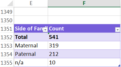
Count by Side of Family Results
Count by Complete Downloads
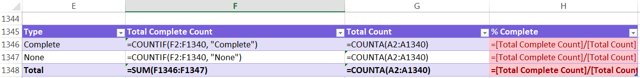
Count by Complete Download
For example, to count the Complete Download, the formula is =countif(Range of Data, “Complete”). The formula will count all cells that contain the word “Complete” from the data table. Then count the total number of rows by with the CountA formula, written as: =counta(range of data). In the last column, divide the Total Complete by the Total Count to get the percentage completed.
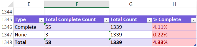
Count by Complete Downloads Results
Count by Relationship Type
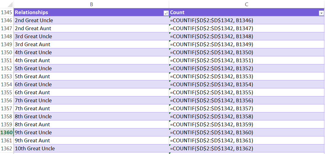
Count by Relationship Type
For example, to count the number of 2nd Great Uncles, the formula is =countif(Range of Data, Cell with the phrase “2nd Great Uncle” in it). The formula will count all cells that contain the matching phrase from the data table.
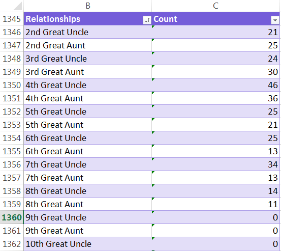
Count by Relationship Type Results
A note about the “$” in some of the formulas: this hard codes the cell referenced in the formula, so that if you drag the formula down to copy it to additional cells, that part of the formula remains constant and only the non-$ numbers adjust.
So many thanks to Michele Simmons Lewis for the inspiration to riff off in order to get organized with my research.
Hi looking for a template link?
here you go! https://rootsofkinship.com/resources/ancestry-document-management-template/
how did you make the excel sheet work with the relationship calcuator I am a newbie to excel
Hi – I didn’t actually calculate the relationship myself, but am using information from Ancestry.com to determine how they are related to me
Larisa,
I’d like to let you know that your blog post is listed in my Fab Finds post at http://janasgenealogyandfamilyhistory.blogspot.com/2015/08/follow-friday-fab-finds-for-august-28.html
Have a great weekend!
Thanks Jana – appreciate being included in such fine company!
I could not get this to work….HELP please!
What are problem are you encountering? I can try to help.
I love your spread sheet. I too am an excel geek. One have added some great features. Do you have it available for download?
I don’t right now, but I’ll make some modifications later today and post a template.
Hi Todd – I just added the template here